Brian Kantor – Page 10

Rising pay-out ratios (dividends/earnings) – half full or half empty for the SA economy?

JSE dividends (All Share Index dividends per share) have increased significantly faster than earnings over recent years. The payout ratio (dividends/earnings) that averaged about a steady 40% between 1995 and 2016 has increased to about 60% of earnings. If we leave Naspers, now about 18% of the All Share Index, out of the calculation, the payout ratio is now close to 70% of reported headline earnings. This ratio is unusually high by international and emerging market comparisons.

Since 2012 JSE dividends per share in rands have doubled while reported earnings are only 20% higher than they were in 2012. Share prices are about 100% up on 2012 levels and have tracked dividends more closely than depressed earnings. A value gap between dividend flows and the price paid for these dividends has opened up. Our model of the JSE indicates that the JSE may be about 15% below its ‘fair value” as predicted by reported dividends and interest rates (see figure below)

Fig.1 JSE All Share Index, earnings and dividends per share (2012=100)

Source; Ires and Investec Wealth and Investment

JSE dividends and earnings are currently growing at about the same rate of about 13% p.a. and are forecast to sustain growth rates of about 10% p.a over the next twelve months. (see chart below)

Fig.2 JSE growth in All Share Index earnings and dividends per share

Source; Ires and Investec Wealth and Investment

Should shareholders welcome or disdain this higher payout ratio? If a company has prospective returns from its investment programme that exceed its cost of capital, it should retain all the cash it is generating and invest it back into the company on behalf of its shareholders. Shareholders can only hope to achieve lower market related, risk adjusted returns with the cash distributed to them. If the company can beat this opportunity cost of capital, it should not pay dividends or buy back its shares. Indeed in such circumstances free cash flow ( cash retained after capital expenditure) will ideally be negative rather than positive. A true growth company would be well justified in raising fresh equity or debt capital to fund its expansion and be revalued accordingly with sustainably faster growth in mind.

That SA companies are paying out more of their earnings is both good news and bad news for shareholders and the economy at large. The good news is that paying out more is better than undertaking capital expenditure, including mergers and acquisitions, that cannot be expected to beat their cost of capital and add value for shareholders .

The attempts SA companies have made seeking growth offshore have often proved value destroying rather than value adding. Such attempts typically add unwanted complexity to SA businesses and reduce their value. While they may diversify away some SA specific risks, shareholders are fully able to undertake their own diversification investing directly in offshore companies. They do not need SA managers to do it for them and venture outside their area of competence.

The bad news implication of higher SA payouts is that it reflects an understandable reluctance to invest more in what has become very slow growth South Africa. Such a reluctance to invest more in capital or people (also called working capital) while good for shareholders, inevitably reinforces the slow economic growth under way.

The solution to the problem of high pay outs in South Africa is to get growth going again. Companies will then invest more in growing markets for their goods and services and retain more cash to the purpose. They would be doing more good for shareholders, their customers, their employees and the wider economy.

It is unrealistic to expect SA firms to invest more unless the markets for what they produce can also be expected to grow. It is the spending of SA households that determines the path of the SA economy. It is the consumption egg that leads the investment chicken.

Without the stimulus of lower interest rates household spending will remain subdued. We can only hope a stronger rand and consequently less inflation will allow the Reserve Bank to help the economy along – rather than stand in its way.

Inflation of prices and wages – have they had any predictable consistent influence on output and employment in the US since 1970?

21^st January 2019

Benign expectations of inflation and interest rates despite low rates of unemployment

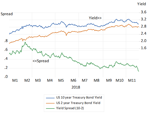
The US capital market in January 2019 reveals a very benign view of inflation and of the direction of interest rates. The long- term bond market indicates that inflation is expected to stay below an average 2% per annum over the next ten years. The difference between the yield on a vanilla 10 year Treasury on January 9^th (2.71% p.a) and an 10 year Inflation protected US bond that day (0.833% p.a) is an explicit measure of inflation expected in the bond market. This yield spread gives long term investors in US Treasuries a mere 1.88% p.a extra yield for taking on the risk that inflation will reduce the real value of their interest income. And the Fed is confidently expected not to raise short term rates this year. The money market believed in January 2019 that there was only a one in four chance of the Fed Funds rate rising by 25 b.p. this year. On January 9^th 2019, the one year treasury bond yield of 2.59% p.a. was expected to be only marginally higher, 2.66% p.a in five years. [1]

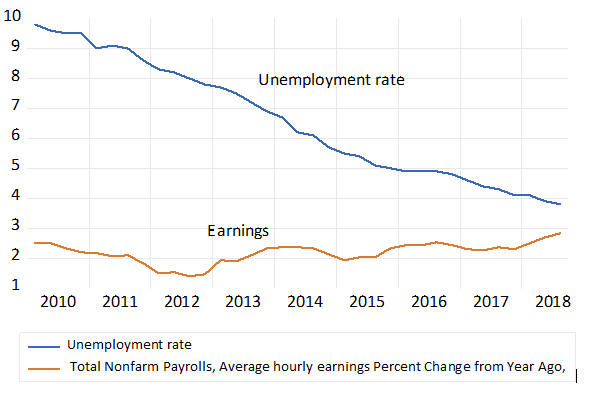
Are such views consistent with a very buoyant labour market it has been asked? Unemployment rates are at very low levels, below 4% of the labour force while average earnings are rising at about 3% p.a. These bouyant conditions in the labour market may portend more inflation and higher interest rates to confound the market consensus.

Fig. 1: The US Treasury Bond Yield Curve on January 9^th 2019.

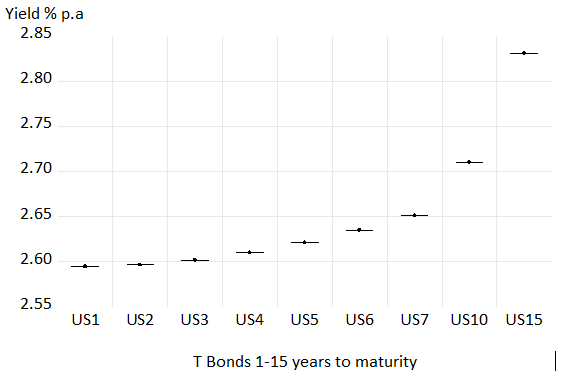
Source; Reuters-Thompson and Investec Wealth and Investment

Figure 2; Unemployment and earnings growth in the US

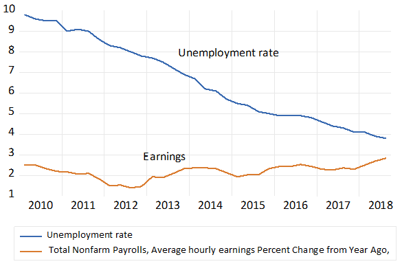
Source; Federal Reserve Bank of St.Louis, Fred data base and Investec Wealth and Investment

The relationship between wages and prices in the US

Do changes in prices lead or follow changes in wage rates in the US? The economic reality is that they both follow and lead. Both the price of labour – average wages and other benefits per hour of work and its cost to employers- and the price of a basket of goods and services, represented by the CPI, are determined more or less simultaneously and inter-dependently in their market places. As we show below the index of average wages and the CPI are highly correlated. How they interact is not nearly as obvious and may not be consistent enough to make for any convincing evidence of cause and effect- that is from prices to wages or wages leading prices.

The relationship between wages and prices and employment and GDP

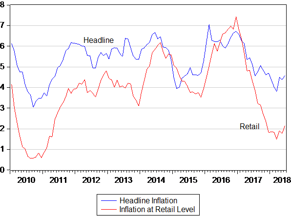
Fig.3 Wage and headline inflation in the U.S 1970-2018.3; Quarterly data, year on year percentage changes

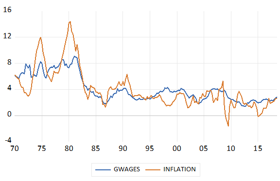
Source; Federal Reserve Bank of St.Louis, Fred data base and Investec Wealth and Investment

As may be seen in the chart above wage inflation in the US ( year on year per cent changes in hourly earnings) appears to track headline inflation very closely and vice versa. Wage inflation has been less variable than headline inflation ( year on year change in the CPI) Headline inflation since 1970 has averaged 4.09% with a standard deviation (SD) of 2.95% p.a. while average wage inflation per annum has been a very similar 4.09% p.a, with a lower SD of 2.02% p.a.

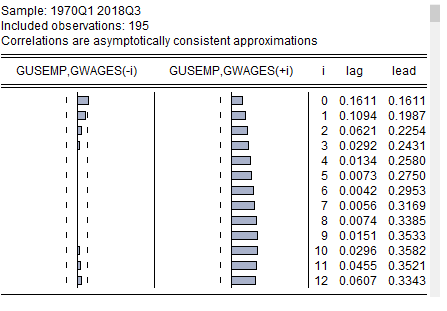
We show below a table of correlations of headline and wage inflation at different leads and lags. As may be seen the highest correlations are realized for contemporaneous growth rates. The correlations remain very similar for lags up to 12 quarters and point to no obviously important and reliable leads and lags that could inform any wage plus theory of inflation.

Table 1; Cross-Correlogram of inflation and growth in wages in the US. Quarterly data Y/Y percentage growth (1970.1-2018.3)

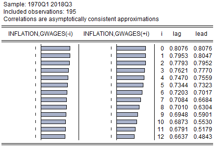
Source; Federal Reserve Bank of St.Louis, Fred data base and Investec Wealth and Investment

Fig.4 Growth in employment and GDP Quarterly data y/y percentage growth (1970.1-2018.3)

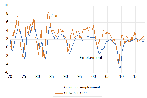
Source; Federal Reserve Bank of St.Louis, Fred data base and Investec Wealth and Investment

We show the very close relationship between the growth of payrolls and the growth in the U.S economy in the chart above. GDP has grown on average by 2.77% p.a since 1970 while employment has increased by 1.56% p.a on average since then. The correlation of the two growth series is 0.60 while, as may be seen, employment growth (SD 1.87% p.a) has been less variable than output growth (SD 2.18% p.a) GDP growth very consistently leads employment growth. The lag effect seems strongest at two quarters. The correlation between changes in GDP and changes in employment two quarters later is as high as 0.86.

We show the lag structure in the Cross-Correlogram below

Table 2. Cross-Correlogram of Growth in Employment and Wages in the US. Quarterly data y/y percentage growth (1970.1 2018.3)

Source; Federal Reserve Bank of St.Louis, Fred data base and Investec Wealth and Investment

Why changes in wage rates and prices are so highly correlated

The markets for goods and the markets for labour have the general state of the economy in common. The wages and prices that emerge in the markets for labour and goods and services will be influenced by how rapidly the demand for and the supply of all goods, services and labour may be growing. Furthermore higher wages or prices will in turn restrain demands for labour and other goods and services effecting the observed wage rate and employment outcomes in the labour market.

Changes in prices, wages and interest rates have their causes (represented in the conventional supply and demand analysis by leftward or rightwards shifts in the demand and supply curves that cause prices to rise or fall) But any such shock to prices or wages or interest rates and asset prices will also have effects on demand or supply, as prices move higher or lower. Such effects can be represented by movements along the relevant demand or supply curves.

The essence of any helpful analysis of supply and demand forces at work is to recognize and identify the sequence of events that lead to any new equilibrium price when supply and demand are again in balance . That is to identify the initial causes of a price change, the supply side or demand side shock that gets prices or wages or interest rates moving in one or other direction, and their subsequent effects on prices and the further adjustments made by buyers and sellers to the shocks. An unexpected spurt of economic growth may well lead to more employment and higher real wages. That is cause a shift rightwards in the demand curve for labour. Higher real wages then serve to ration the available supply of labour under pressure from increased demands.

These higher wages may induce more potential workers to seek employment. Such responses would make the supply curve of labour more elastic in response to higher wages. Thus more worker employed will help offset the initial wage pressures emanating from the demand side of the market .

Supplies of goods and services and capital and labour may also come from abroad to add to supplies and so influence prices on the domestic markets. Trade and capital flows may alter the rate of exchange that, depending on their direction, may add to or reduce the price of imports in the local currency. And exports can add to demands – so competing with local buyers and to possibly price them out of the local market. It is demand and supply that determine prices and wages. The changing state of domestic demand may not be enough to push prices or wages consistently higher. The final outcomes for prices will also depend on the supply side responses.

Furthermore prices are not simply set as a pre-determined percentage higher than the cost of producing them. Of which the costs of employing workers may be a more or less important part, depending on the labour intensity of production. The state of the economy (demand) and the competition to supply customers will determine how much margin over costs will their way into the prices any firm will charge.

Costs to some firms are the prices charged by their suppliers- including their employees. The distinction between what may be described as costs, or alternatively prices, will be based on the position the buyer or seller occupies in the supply chain. In the very long run prices and the costs of supplying all goods or services offered will tend to converge. The relevant cost to be covered will include the opportunity costs of employing capital as well as labour.

Is it a matter of demand pull or cost push on prices- or is it both – with variable difficult to predict lags between prices and costs or costs and prices? The evidence of wage and price growth trends says it is both as would any full theory of wage and price determination.

Another force common to prices wages and interest rates is the increase in prices and wages expected in the future. The faster they are expected to increase the more workers and firms and investors for that matter will wish to charge upfront for their services. All this complexity makes any uni-directional wage or cost-plus theory of inflation of very limited explanatory or predictive power.

The Phillips curve – origins and uses.

There is an economic theory known as the Phillips curve, that predicts that decreases in the unemployment rate (increases in the demand for labour) would cause wages to rise faster and for prices and interest rates to follow. The original paper written in 1958[2] was primarily an exercise in innovative, early econometrics. It demonstrated how curves could be fitted to annual data on changes in wages and the unemployment rate. It showed a broadly negative relationship between wage rates and the unemployment rate. The theory was that increased demands for labour- represented by a lower unemployment rate -would lead to higher wages.

The data extended over a long run, 1861-1957. It was collected over a period when the United Kingdom was mostly on the gold standard and when inflation would have been confidently expected to be sustained at very low levels. Of interest is that Phillips in his paper was well-aware of the role variable import prices might play in influencing prices and wages. A force we would describe today as a supply side shock.

It was this theory that Keynesian economists invoked in the sixties to argue that more employment could be traded of for more inflation. The idea was that workers, unwilling to accept the wage cuts that might restore full employment, might be fooled by inflation that surreptitiously reduced their real wages and so encouraged employment. Employment opportunities that were presumed to be structurally deficient – depression economics that is.

The classical economists regarded the flexibility of wages and prices in the downward direction as the cure for recessions. The extended unemployment of the nineteen thirties appeared to indicate that any reliance on wage and price flexibility to restore full employment was unrealistic. Given that nominal wages were seen as rigid in the downward direction meant persistently high levels of unemployment. That is unless governments intervened to stimulate aggregate demand enough to cause inflation and thereby reduce real wages enough to encourage employment. The implications of the Phillips curve that appeared to trade higher nominal wages for more employment was generalised to imply a tradeoff of inflation for faster growth.

The predictive powers of the Phillips curve

The theory has had very poor powers of prediction- originally of what became high inflation and slower growth in the US and elsewhere in the nineteen seventies. Much higher average rates of inflation of prices and wages in the seventies were associated with much slower not faster growth. This lethal combination came to be described as stagflation. That inflation was accompanied by slower not faster growth encouraged monetarists with an alternative demand led rather than a wage led theory of inflation. The quantity theory of prices, reconfigured by Milton Friedman, regained its currency. [3]

Any negative relationship between wages and unemployment (increased wage rates associated with less unemployment or more generally more inflation associated with faster GDP growth) in the US is conspicuously absent in the employment inflation wage growth and GDP data ever since the 1970’s and in-between. We demonstrate the absence of any support for the Phillips curve in the charts and tables below.

As may be seen the scatter plots and the regression lines that connect them indicate that unemployment and wage increases and inflation and GDP growth are not related in any statistically significant way. This is true of the relationship between unemployment (or employment) over the entire period 1970 – to 2018 and sub-periods including more recently between 2000 and 2018 and between 2010 and 2018. The correlations for the entire period and for sub-periods within them between wage growth and employment growth and between inflation and output growth are close to zero as may be seen in the table of regression results. The scatter plots and their regression lines shown below indicate the absence of any consistently meaningful relationships very clearly.

The table of regression results shown below confirms the absence of any predictable statistically significant relationship between employment and wage growth or between GDP growth and prices or indeed vice-versa. As may be seen the single equation regression equations are almost all explained by their alphas. The goodness of the fits of the regressions are very poor indeed. Their respective R squares that are all close to zero- indicating that the growth rates are generally not related at all. The betas that determine the slope of the regression lines are of small magnitude and most do not pass the test of statistical significance at the 95% confidence level – and some that do, for example equations 6 and 11, indicate that the relationship between wage growth and employment is a negative rather than a positive one. The presence of serial correlation in the equations as demonstrated by the Durbin-Watson (DW)statistic indicates that these betas may well be biased estimates. It would seem very clear that there is no trade-off between wage and price growth and the growth in output and employment in the US. Any forecast hoping to predict inflation via recent trends in wage rates or employment would be ill-advised to do so, given past performance.

Fig.5; Inflation and growth in real GDP Quarterly Data Growth year on year. Scatter Plot and Regression line (1970.1 2018.3)

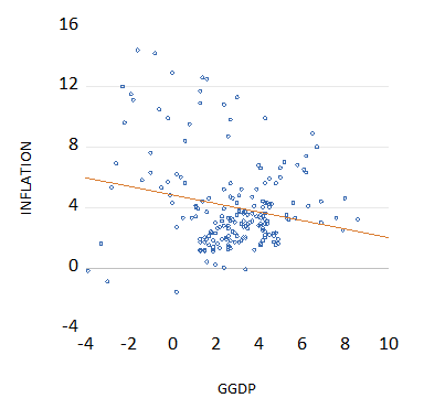
Source; Federal Reserve Bank of St.Louis, Fred data base and Investec Wealth and Investment

Fig 6: Growth in wages y/y and the unemployment rate 1970.1 2018.3 Scatter Plot and regression line

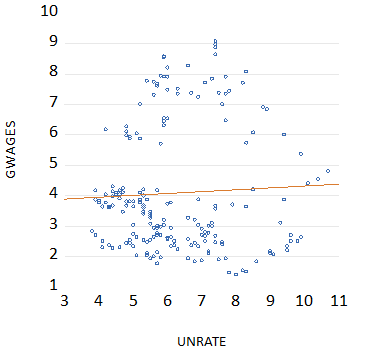
Source; Federal Reserve Bank of St.Louis, Fred data base and Investec Wealth and Investment

Fig.7; Growth in wages and growth in employment (1970,1 2018.3) Scatter Plot and regression line

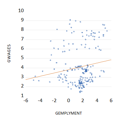
Source; Federal Reserve Bank of St.Louis, Fred data base and Investec Wealth and Investment

Fig.8; Inflation and growth in GDP (1970-79) Scatter Plot and regression Line

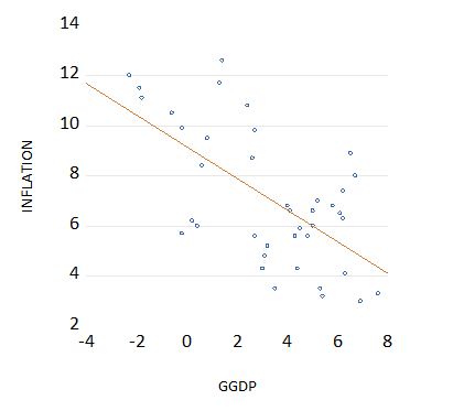
Source; Federal Reserve Bank of St.Louis, Fred data base and Investec Wealth and Investment

Fig 9; Growth in wages and unemployment rate (2010.1 2018.3) Scatter Plot and regression line

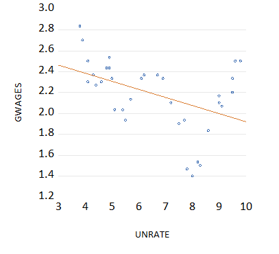
Source; Federal Reserve Bank of St.Louis, Fred data base and Investec Wealth and Investment

Table 2; Regression results

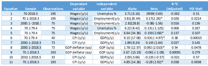
[4] The data is downloaded from the St Louis Federal Reserve data base Fred. The data is quarterly and seasonally adjusted and all growth rates have been calculated by Fred and downloaded into Eviews. Eviews was used to run the regression equations and construct the charts. Wages were represented by average hourly earnings of production and nonsupervisory employees in the private sector. (AHETP) Employment by Total Nonfarm Payrolls (PAYEMS) The unemployment rate (UNRATE) is the civilian unemployment rate. The GDP and CPI have their conventional descriptions

Not inflation- only unexpected inflation has real effects on output and employment

That is because firms and workers build inflation into their wage and price settings. Much faster inflation in the seventies did not come to surprise workers and did not mean lower real wage costs for the firms that hired them. Moreover prices rise faster as they did in the seventies, as the oil price rose so dramatically, when Middle East producers exercised their newly found monopoly power to restrict supplies. Negative supply side shocks that raise prices and reduce demand will complicate the relationship between price and wage changes.

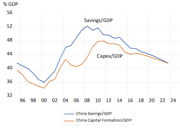
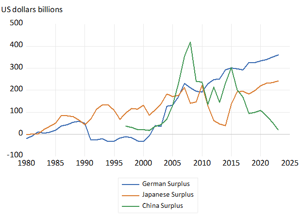
A larger positive supply side shock for the global economy that caused downward pressure on prices was the entrance of China and Chinese labour and enterprise into the global economy. It brought a very large increase in the supply of goods- especially of manufactured goods. This addition to supplies at highly competitive prices lowered the prices established producers outside of China have been able to charge and forced many of them out of business.

The challenges for the economic forecaster

It is possible to build more complex multi- equation models that incorporated lags between GDP growth and employment growth and between changes in prices and wages to hopefully forecast inflation and growth. That is consistently with economic theory combined supply and demand forces and their feed-back effects with due importance attached to inflationary expectations and how they are established. If the feed-back effects however accurately identified are themselves of variable force through different phases of the business cycle the estimates of the equations are unlikely to deliver statistically meaningful results.

The accuracy of such forecasts will depend not only on the internal logic of the equations estimated, but on the assumptions made about the forces outside the model. The predictive power of such models must be tested out of the sample periods over which the coefficients of the model were estimated. Forecasters inside and outside of central banks have every incentive to make accurate forecasts of inflation, growth, interest rates and asset prices. The ability of any of these models to consistently beat the market place has to date never been obvious. And were they so able the market itself would become less volatile.

Inflationary expectations and the reactions of central bankers[5]

The importance of inflationary expectations in the determination of the price and wage level has much impressed itself on central bankers. They recognized that there was no output or employment benefit to be gained from more inflation. That only unexpectedly higher inflation might stimulate more output- and unexpectedly low inflation will do the opposite. The central bankers have come to understand that their ability to surprise the market and their forecasts is very limited. Given that is the importance workers (trades unions)and firms with price or wage setting powers would attach to predicting inflation as accurately as possible. They do so in order to avoid the potential income-sacrificing consequences of underestimating or over estimating inflation. Underestimating the inflation to come would mean setting wages and prices below where market forces might have justified. Overestimating inflation might mean wages and prices having to reverse direction with a consequent loss of output and employment. Successfully second -guessing central bank action that helps determine the rate of inflation is an essential ingredient for successful market makers.

When the surprises are revealed they will come with losses of output and employment as the market adjusts or in the case of surprisingly rapid inflation exchange rate weakness and higher interest rates will follow. Dealing with such surprises adds volatility to prices and asset prices. A risky environment discourages savings, inward capital flows and investment and reduces potential output and its growth.

Thus central bank wisdom is that they should avoid as far as possible inflation shocks and associated monetary policy actions that might surprise the market place. Rather they have come to understand that their task is offer the market place a highly predictable and low rate of inflation in the interest of permanently faster growth rates. Hence inflation targeting.

A South African post-script

This is the objective of the SA Reserve Bank -enshrined in our constitution – as we have been well reminded recently. But success in achieving balanced growth does demand more flexibility than the SA Reserve Bank has demonstrated. The flexibility to recognize that powerful and frequent supply side shocks to inflation – exchange rate, oil price and food price shocks call for very different interest rate responses than when demand is leading inflation.

Alas demand led inflation has been conspicuously absent in recent years. Wage increases in SA therefore explain unemployment not inflation. Accurately forecasting inflation in SA – better than the Reserve Bank has been able to do – means anticipating the exchange rate and the oil price and rainfall in the maize triangle. A near impossible task it may be suggested. Eliminating demand led inflation ( policy settings that attempt to balance domestic demand and supply) rather than directly aiming at an inflation rate that is largely beyond its control is a much more realistic and appropriate task for the SA Reserve Bank. And the market place can fully understand these realities. Inflation forecast and so inflationary expectations in SA will be rational ones.

[1] By Reuters-Thompson interpolating the yield curve that is reproduced here

[2] A.W.Phillips, The relationship between unemployment and the rate of change of money wage rates in the United Kingdom, 1861-1957,Economica vol 25 (19580 pp 283-99

[3] My own interpretation of the analytical disputes of the time can be found in my Rational Expectations and Economic Thought, Journal of Economic Literature, Volume XV11 9December 1979),pp 1422-1441 it referred to the pioneering work on the role of expectations in macro-economics of Milton Friedman (1968) and Edmund S.Phelps (1967 and 1970)

[4]

[5] See my, The Beliefs of Central Bankers about Inflation and the Business Cycle—and Some Reasons to Question the Faith, Journal of Applied Corporate Finance; Volume 28, Number 1, Winter 2016

Inflation and balanced growth – taking the market seriously

The bond market indicates that inflation is expected to stay below 2% per annum over the next ten years in the US. And the Fed is confidently expected not to raise short term rates this year.

Are such views consistent with a very buoyant labour market? Unemployment rates are below 4% while average earnings are rising at about 3% p.a. Some believe this portends more inflation and higher interest rates that will confound the market consensus.

U.S. Unemployment rate and growth in earnings

Source; Fred- Federal Reserve Bank of St.Louis and Investec Wealth and Investment

Do changes in prices lead or follow changes in wage rates in the US? The economic reality is that they both follow and lead with variable lags. The markets for goods and the markets for labour have the general state of the economy in common. The wages and prices that emerge depend upon how rapidly the demand for and the supply of all goods, services and labour are growing. Higher or lower prices, wages and asset valuations have their causes and in turn will have effects on the willingness to buy or sell. And might not higher real wages in the US soon reduce the demand for labour and employment – as they have done in SA?

The prices of goods and services are not simply determined by adding a constant percentage point to the cost of producing them. The state of the economy (demand) and the competition to supply customers (including from abroad) will determine how much margin over costs finds its way into the prices a firm will charge. It is this mix of demand pull and cost push and pressures on margin that determines prices.

Another force common to both is the increase in prices and wages expected in the future. The faster they are expected to increase the more workers and firms and investors will wish to charge upfront for their services.

The Phillips curve predicts that decreases in the unemployment rate (increases in the demand for labour) will cause wages to rise faster. Keynesian economists invoked this theory in the sixties to argue that more employment could be traded of for more inflation that comes with higher wages. The idea was that workers, unwilling to accept the wage cuts that might have restored full employment, might be fooled into accepting lower real wages by inflation.

The theory has had very poor powers of prediction- particularly in the high inflation and slow growth seventies. It became a case of more inflation and slower growth and still is. Firms and workers and the unions that negotiate for them have every reason to build inflation into their wage and price settings. Therefore only inflation surprises therefore can have real effects on the economy- not inflation itself.

And the market place is not easily surprised. Their inflation forecasts, using very similar methods, are as likely to be accurate or rather as inaccurate as those of the central banks. There is no good reason to believe that any wage plus theory of inflation will beat the market view on inflation today.

Central bankers have long recognized that there was no output or employment benefit to be gained from tolerating more inflation. Only unexpectedly higher inflation might stimulate more output- but the ability of monetary policy to helpfully surprise the market is very limited. Central bankers now judge it better to avoid inflation surprises in both directions. Better they believe to offer the market place a highly predictable and low rate of inflation in the interest of balanced and permanently higher growth rates- as does the SA Reserve Bank.

Yet balanced growth demands more flexibility than the SA Reserve Bank has demonstrated. The flexibility to recognize that powerful and possibly frequent supply side shocks to inflation – exchange rate, oil price and food price shocks – do not call for higher interest rates. Central banks can hope to stabilize aggregate demand – supply management is beyond their compass. And the market place is fully capable of recognizing the difference. Inflationary expectations are also rational.

January 9th 2019

If you could borrow as much as might wish at close to zero rates of interest for ten or more years you would surely do so. There would be no lack of projects that promised wealth generating returns of at least one per cent p.a. Of course such funding opportunities are not readily available to any ordinary business or household. Lenders would demand a premium to cover risks of default and would raise the prospective returns potential investors would have to achieve.

But such considerations do not apply to the German, Japanese, Netherlands or even the Brexit stressed UK government or the Swiss that can borrow at negative rates of interest. Lenders pay for the privilege of funding the Swiss government – for ten years and more. These governments can borrow as much as they might wish at very low rates.

Surely an extra bridge or highway, port or pipeline or even a dyke helping to create a productive polder can promise a one per cent per annum return? Governments with such favourable credit ratings neither have to undertake the construction nor the management of such low return projects that can be leased to private operators- who win competitive tenders to do so. And if governments would exercise such opportunities to borrow more at invitingly low rates – also, heaven forbid, to cut income and expenditure tax rates – aggregate demand for goods and services would be stimulated. And businesses would add to their productive capacities, including their work forces. And depressed rates of growth of GDP and accompanying incomes would accelerate.

Demands for credit especially bank credit would be encouraged, bank balance sheets would strengthen, while the national savings rates declined and interest rates could rise for very good reasons. Because demands for capital to invest would be rising rise faster than supplies of savings.

The failure to respond to respond sensibly to an extraordinary level of savings and the accompanying low interest rates is the essential European economic problem. The rate at which the Germans have saved has increased dramatically since 2000, while the rate at which they have added to their stock of capital fell away.

Germans in 1995 saved about 22% of their incomes- a very high rate for a developed economy. They are now saving 28% of their very large GDP that is forecast to rise further.They add to their capital stock at a 20 per cent of GDP rate. This has meant dramatically larger flows of capital out of Germany into global capital markets. In 2018 outflows of about 400 billion dollars were estimated.

Savings and Capital Formation ratios to GDP in Germany. Annual data

Source; IMF World Economic Outlook 2018 and Investec Wealth and Investment

The Dutch are now saving a similarly high proportion of their incomes and the Japanese are a further major source of global savings. The Chinese save at an even higher rate, over 40% of GDP, though the rate at which savings are made and capital formed has been falling. China is no longer a significant contributor to the global savings pool. A fact that may well inhibit its ability to stimulate its economy.

China – saving and capital formation to GDP ratios. Annual data

Source; IMF World Economic Outlook 2018 and Investec Wealth and Investment

Contribution to global capital markets. The combined surpluses of Germany, Japan and China (US dollar billions)

Source; IMF World Economic Outlook 2018 and Investec Wealth and Investment

The contribution in 2007 to the global savings pool from China, Germany and Japan amounted to nearly a trillion US dollars – compared to about a mere $100b seven years before. It is now about $600b.

The borrowers to absorb these surpluses at low interest rates were naturally found in the credit hungry US. Inflows of capital to the US expanded dramatically after 1995 – much of it funding houses that had to be abandoned by their owners after 2008. The average US home lost 30% of its pre-global financial crisis value. No mortgage based financial system could hope to survive a collapse in asset values of this magnitude- without a bail out.

US capital inflows 1980- 2023 – A tale of growing dependence.

Source; IMF World Economic Outlook 2018 and Investec Wealth and Investment

Less not more austerity is urgently called for in northern Europe- to help save the euro and the European project. The Italian and other populists are on the right track while the German fiscal conservatives perversely continue down a dead end.

The market rules OK?

December 5, 2018

The global financial markets are reacting to two forces at work. About what Fed Chairman Powell might do to the US economy with interest rates and what President Trump might do to the Chinese economy with tariffs.

Interest rates set by the Fed might or might not prove helpful for the US economy. Given its unknown future path. It is not Potus but market forces that are restraining interest rate increases in the US. The absence of which is helpful to share prices- all else, expectations of earnings growth for example, remaining unchanged.

It is the US bond market itself that has eliminated any rational basis for the Fed to raise short term interest rates. Should the Fed pursue any aggressive intent with its own lending and borrowing rates, interest rates in the US market place, beyond the very shortest rates, are very likely to fall rather than rise.

Hence the cost of funding US corporations that typically borrow at fixed rates for three or more years and the cost of funding a home that is mostly fixed for twenty years or more, would likely fall rather than rise. And so make credit cheaper rather than more expensive.

The term structure of interest rates in the US has become ever flatter over the past few months. The difference between ten-year and two-year interest rates offered by the US Treasury has narrowed sharply. Ten year loans now yield only fractionally more (0.13% p.a) than two year loans. (See figure below)

Fig.1: Interest rates in the US and the spread between ten year and two year Treasury Bond yields

Source; Bloomberg and Investec Wealth and Investmment

This difference in the cost of a short term and long term loan could easily turn negative- that is longer term interest rates falling below short rates should the Fed persist with raising its rates. Which it is unlikely to do beyond the 0.25% increase widely expected in December for term structure reasns.

The US capital market is not expecting interest rates to rise from current levels in the future. Given the opportunity to borrow or lend for shorter or longer periods at pre-determined fixed rates, the longer term rate will be the average of the short rates expected over the longer period. Lending for two years at a fixed rate must be expected to return as much as would a one year loan- renegotiated for a further year at prevailing rates. Otherwise money would move from the longer to the shorter end of the yield curve or vice versa to remove any expected benefit or cost.

By interpolation of the US treasury yield curve, the interest rate expected to be paid or earned in the US for a one year loan in five years time, has stabilized at about 3.2% p.a. or only about 0.5% p.a more than the current one year rate. These modest expectations should be comforting to investors. They are not expectations with which the Fed can easily argue- for fear of sending interest rates lower not higher.

Fig.2; US One year rates expected in five years

The market believes that interest rates will not move much higher because market forces will not act that way. Increased demands for loans at current interest rates – are not expected to materialize. They are considered unlikely because real growth in the US is not expected to gain further momentum and is more likely to slow down from its recent peak rate of growth. Furthermore, given the outlook for real growth, inflation is unlikely to pick up momentum. For which lenders would demand upfront compensation in the form of higher yields.

The market of course might change its collective mind – redirecting the yield curve steeper or shallower. And in turn giving the Fed more or less reason to intervene helpfully. Interest rate settings should not unsettle the market place. They are very likely to be pro-cyclical

But the more important known unknown for the market will be Donald Trump and his economic relationship with the rest of the world. Perhaps Trump himself can also be helpfully constrained by the market place. The approval of the market place can surely help his re-election prospects.

Retailers give thanks for Black Friday — and all of December

As published in the Business Day on 23 November 2018: https://www.businesslive.co.za/bd/opinion/columnists/2018-11-23-brian-kantor-retailers-give-thanks-for-black-friday–and-all-of-december/

It was Thanksgiving in the US on Thursday, a truly interdenominational holiday when Americans of all beliefs, secular and religious, give thanks for being American, as well they should.

This is a particularly important week for US retailers. They do not need to be reminded of the competitive forces that threaten their established ways of doing business. Nor do investors who puzzle over the business models that can bring retail success or failure.

The day after Thanksgiving is known as Black Friday, when sales and the profit margins on them will hopefully turn their cumulative bottom lines from red to black. It has been Black Friday all week and month and advertised to extend well into December. Presumably, to bring sales forward and make retailers less dependent on the last few trading days of the year.

As we all know, competition has become increasingly internet- based from distributors of product near and far and yet only a day or two away. E-commerce sales have grown by over three times since 2010, while total retail sales including e-commerce transaction are up by half since 2010. Total US retail sales, excluding food services, are currently more than $440bn and e-commerce sales are over $120bn. The growth in e-commerce sales appears to have stabilised at about 10% per annum.

The importance of online trade is conspicuous in the flow of cardboard boxes of all sizes that overflow the parcel room of our apartment building, including boxes of fresh food from neighbouring supermarkets.

The neighbourhood stores of all kinds are under huge threat from the distant competition, which competes on highly transparent prices on easily searched for goods on offer, as well as convenient delivery. As much is obvious from the many retail premises on ground level now standing vacant on the affluent upper East side of New York. The conveniently located service establishments survive, even flourish, while local clothing stores go out of business because they lack the scale (and traffic, both real and on the web) to make a credible offering.

But spare a thought for SA retailers, for whom sales volumes in December are much more important than they are for US retailers. November sales for US retailers — helped by Thanksgiving promotions — are significantly more buoyant than December volumes. According to my calculations of seasonal effects since 2010, US retail sales in December are now running at only 90% of the average month, while November sales are well above average at 116% of the average month.

However, retail sales statistics in the US include motor vehicle and fuel sales, which are excluded from the SA stats. December sales in SA are as much as 137% above the average month, help as they are by summer holiday business, as well as Christmas gifts.

A New York (retail) state of mind

New York, November 21^st 2018

It is Thanksgiving this Thursday in the US – a truly inter-denominational holiday when Americans of all beliefs, secular and religious, give thanks for being American – as well they should.

This is a particularly important week for American retailers. They do not need not to be reminded of the competitive forces that threaten their established ways of doing business. Nor do investors who puzzle over the business models that can bring retail success or failure.

The day after thanksgiving is known as Black Friday, when sales and the profit margins on them will hopefully turn their cumulative bottom lines from red to black. It has been black Friday all week and month and advertised to extend well into December. Presumably, to bring sales forward, that is to make retailers less dependent on the last few trading days of the year.

The competition as we all know has become increasingly internet based from distributors of product near and far, and yet only a day or two away. E commerce sales have grown by over three times since 2010 while total retail sales including E commerce transaction are 50%up since 2010. Total US retail sales, excluding food service are currently over $440b and E commerce sales are over $120b (see figures 1 below)

Fig 1; US Retail and E Commerce sales (2010=100) Current prices

Source; Federal Reserve Bank of St.Louis (FRED) and Investec Wealth and Investment

The growth in E Commerce sales appears to have stabilised at about 10% per annum. (see figure 1)

Fig 2; Annual growth in total retail and E commerce sales in the US (current prices)

Source; Federal Reserve Bank of St.Louis (FRED) and Investec Wealth and Investment

Retail sales of all kinds have been growing strongly – though the growth cycle may have peaked- as may have GDP growth- leading perhaps to a more cautious Fed. How slowly growth rates will fall off the peak is the essential question for the Fed as well as Fed watchers and answers to which are moving the stock and bond markets. (see figure 3)

Fig.3: The US retail growth cycle

Source; Federal Reserve Bank of St.Louis (FRED) and Investec Wealth and Investment

The inportance of on-line trade is conspicuous in the flow of cardboard boxes of all sizes that overflow the parcel room of our apartment building. Including boxes of fresh food from neighbouring supermarkets. The neighbourhood stores of all kinds are under huge threat from the distant competition that competes on highly transparent prices on easily searched for goods on offer as well as convenient delivery. As much is obvious from the many retail premises on ground level now standing vacant on the affluent upper East side of New York. The conveniently located service establishments survive, even flourish, while the local clothing store goes out of business because they lack the scale (and traffic both real and on the web) to offer a credible offering.

But spare a thought for SA retailers for whom sales volumes in December are much more important than they are for US retailers. November sales for US retailers – helped by Thanksgiving promotions – are significantly more buoyant than December volumes. According to my calculations of seasonal effects since 2010, US retail sales in December are now running at only 90 per cent of the average month while November sales are well above average, at 116% of the average month. Retail sales in the US however include motor vehicle and gasoline sales that are excluded from the SA statistics. December sales in SA are as much as 137% above the average month helped as they are by summer holiday business as well as Christmas gifts. (See figure 4 below that shows the different seasonal pattern of sales in the US and SA)

Fig.4; The seasonal pattern of retail sales in SA and the US (2015=100)

Source; Federal Reserve Bank of St.Louis (FRED) and Investec Wealth and Investment

In the black Friday for SA retailers thus comes later than it does in the US. And perhaps makes the case for adding promotions in November to smooth the sales cycle and reduce the stress of running a retail business. They may also hope that the Reserve Bank is not the grinch that spoils Christmas- though the answer to this will come on Thanksgiving.

Unemployment in SA – wishful thinking does not solve the problem

The recent labour force survey of some 30,000 households by Stats SA confirmed the baleful state of the labour market. That is the ever growing mismatch between supply and demand for workers in SA. In the third quarter the supply of potential workers increased, by 153,000 or 0.4% and much faster than the demand for them that increased by 92,000 to 16.4m. The numbers defined as unemployed, not working but actively looking for work, increased by 127,000 to 6.2m pushing the unemployment rate up to 27.5% of the potential work force.

But not all the news from the employment front was bad – depending on your perspective. While the formal sector continued to shed jobs, the informal sector was adding them at a rapid rate. In Q3 informal employment outside of agriculture rose by 188,000 and by 327,000 or 12.2% over the past year to over 3m workers employed informally, or over 18% of all employed.

The decline in formal and the increase in informal employment is not a coincidence. Formal employment has been subject to a rising tide of intervention by government and trade unions (with more to come soon in the form of a national minimum wage) These have provided those in jobs with consistently improved wages and other valuable employment benefits and security to a degree against dismissal and compensation for retrenchment. The informal sector’s employers and workers largely escape these constraints on the freedom to offer and supply employment opportunities. If formal employment – decent jobs as they are described – are unattainable – the choice may be only informal employment or not working or earning much less. A Hobson’s choice that many more South Africans are exercising.

It should be well appreciated that while formal employment, outside the public sector, has stagnated, the share of employment costs in total value added by private business has not fallen. The bill for employment benefits in real terms has gone up in real terms as have employment benefits for those in work, even as the numbers employed have gone down. ( see figures below)

Non-Financial Corporations – Share of Value Added. Operating Surplus and Compensation of Employees

Source. SA Reserve Bank and Investec Wealth and Investment.

Real Value Added by Non-Financial Corporations (1995=100) Using household consumption deflator

Source. SA Reserve Bank and Investec Wealth and Investment.

Non-financial corporations – Growth in Real Value Added and Real Compensation (using household consumption deflator)

Source. SA Reserve Bank and Investec Wealth and Investment.

If the wage bill in any sector of the economy goes up faster than the decline in union membership (as it has been doing) the pool of income upon which to draw union dues is deeper, not shallower. Strikes that increase employment benefits at the expense of employment are therefore not irrational from the perspective of union leaders -if wages increase at a faster rate than employment declines.

The jobs summit would have been better described as the “Decent Jobs Summit” for which the heralded Landmark Framework Agreement is but a wish list of all and everything that can be imagined to promote the demand for labour. A plan however that gives no consideration to the possibility that the rising cost of hiring labour and the more onerous conditions imposed on its hire, may have something to do with the disappointing volume of employment provided.

Everybody will agree that decent jobs for all able and willing to work is to be wished for. And to hope that economic growth can make it possible – as has largely true of employment conditions in the developed world. But the irresistible truth is that far too few South Africans have the skills, the qualifications or experience to allow them to be employed on decent terms- by inevitably cost conscious employers .

And the soon to be imposed National Minimum Wage (NMW) of R3500 per month or R20 per day will make it even more difficult to find employment outside of the informal sector. Because these minimums are well above what many in employment currently earn. And despite the fact that of the poorest in SA the apparent beneficiaries, a very small proportion are currently employed.

For all the many (including economists who should be trained to know better) to wish wages higher and poverty away it has been convenient to ignore the findings of the one comprehensive and highly relevant study. That is the very thorough study by Haroon Bhorat and colleagues of the impact of higher minimums etc. on employment in SA agriculture introduced after 2003. The impact on employment- down 20% -and much improved wage benefits for those still employed – were correctly described by the analysts as significant. There is every reason to conclude that the impact of the NMW on employment will be as significantly and destructive for those who lose their jobs. And helpful for those who retain their jobs on improved terms. They will be even more carefully selected for the skills and strengths they bring to their tasks. The informal sector will have to come to the rescue of the larger numbers of unemployed workers while they wait impatiently for economic miracles.

Ten years after the crash: What has South Africa learnt?

Listen to the Podcast: 10 Years after the crash

It’s a decade since the global financial crisis shook the world’s financial system. The policy response prevented a global depression, but in the process rewrote the textbook on monetary policy. Professor Kantor examines the crisis and the policy response – and then looks beyond, with particular lessons for South Africa.

The backdrop to the global financial crisis

The global financial crisis (GFC) of 2008-09 was caused by the collapse in the value of US homes, as well as the globally-circulated securitised and mortgage debt that had funded a long boom in US house prices. The value of an average US home had increased by an average of 9.2% per year between January 2000 and December 2006. By the time house prices bottomed in February 2012, the average home had lost 32% of its peak value of July 2006. US mortgages on the balance sheets of banks around the world – not only in the US – had lost much of their once-presumed secure value. As a result, much of the capital of the highly leveraged banks was wiped out.

South African banks cannot flourish without a strong economy. Similarly, the economy cannot flourish without real growth in the supply of money and credit. Both have been lacking recently as we show in figure 1 , where we relate real economic growth to the real money and credit supply.

As was the case between 2003 and 2008, it will take a combination of better export prices, a stronger rand, less inflation, and lower short-term interest rates to spark the economy to a cyclical recovery. It will also take more encouraging economic policies for investors in SA businesses (less policy associated risks), including investors in SA banks, to permanently raise the growth potential of the South African economy. There is no reason to believe that South African banks would not be up to the task of funding a much stronger economy. What is required for both are higher returns on capital invested by banks and businesses generally: these would need to be risk-adjusted returns that would justify reinvesting earnings at a faster rate, and raising additional share and debt capital to sustain growth.

The price index of US bank shares peaked in May 2007 and troughed in September 2011, some 70% lower. Average house prices in the US regained their crisis levels by 2013, while the value of the average US bank share exceeded its value of September 2008 a little sooner. The values of both US banks and houses are now above their pre-crisis peak levels, though it took until 2016 or 2017 to get back to the heights of the pre-crisis boom (see figure 1 ).

The crisis for US banks has been long over, thanks to the bold and unprecedented interventions of the US Federal Reserve (the Fed), which pumped extraordinary amounts of cash into the banking system. The US Treasury recapitalised the banks, even those that it was argued didn’t need the helping hand. Europe took longer “to do what it took,” in the famous words of the chairman of the European Central Bank (ECB), Mario Draghi, but largely succeeded in securing its banking system. The central banks and treasuries of Japan and the UK ran their own similar rescue operations.

South African banks were not directly exposed to the US mortgage market, although those with significant exposures offshore felt more of the draft. This was because the South African housing market held up well enough in its relevant rand value after 2008 to prevent any major write-downs of the value of the mortgage credit provided by the banking system. The price of the average middle-class house maintained its rand value after the GFC, while the fall in the value of the banks listed on the JSE was less severe than in the US.

South African banks and other financial institutions were, however, damaged collaterally by the collapse in the share prices of banks and financial institutions in the developed world. They were also damaged by sharp declines in the value of corporate and government debt, including South African government debt held on their balance sheets. The rand value of the JSE Banks Index declined by about 43% from its peak of April 2007 to its trough in February 2009 (see figures 2 and 3 in link ).

The impairment ratio of SA banks fell sharply between 2003 and 2007, but then rose sharply to ratios of about 2.4% to 2.8% of credit provided. These ratios have been more or less maintained since 2010.

The South African Reserve Bank did not practice quantitative easing (QE), which are efforts to avert a liquidity crisis by pumping cash into the banking system through the purchase of government bonds and other securities in the market on a truly massive scale. Nor did the South African Treasury have to recapitalise the system by subscribing to additional share or debt issued by banks and insurance companies, as did the US government and the European Central bank.

Much of the extra cash supplied to the banks of the US, Europe and Japan ended up on the asset side of their balance sheets as deposits with their central banks. The scale of these bank deposits with their central banks grew to be well in excess of the cash reserves they were required to hold against deposit liabilities. The extra cash supplied by central banks to their member banks was held as cash rather than used (as would have been usual) to fund bank loans or investments. Holding excess cash reserves that usually earn no interest is not profitable for banks, though the US Fed offered interest on these deposits. The other central banks do not do so, and the ECB charged banks to hold deposits.

The extra spending normally associated with additional cash supplied to banks thus did not materialise. This was because the extra cash supplied to the banking systems was closely matched by extra demands for cash. Inflation was restrained accordingly, in response to QE. Indeed, central bankers worried more about deflation than inflation after the crisis, a concern that encouraged still more QE until 2015. Only then did the Fed balance sheet stop increasing. A reversal of QE – reduced central bank holdings of assets – is still to transpire in Europe or Japan.

In figures 5 and 6 we demonstrate QE in action in the US. Note the increase in the size of the Fed balance sheet – from less than US$1 trillion in 2008 to over US$4 trillion by 2014. Note also the equivalent increase in cash reserves (deposits with the Fed) of close to an extra US$3 trillion – almost all of which were in excess of required reserves. Cash supplied by a central bank is described as high powered money because it leads to a multiple expansion of bank deposit liabilities (and bank credit on the asset side of the balance sheet of the banks). This is because the cash supplied to the banking system by the central banks is then loaned out by the banks and put to work by the customers of banks.[1]

The contrast with South African banking developments over the same period is striking. The assets of SA banks declined very marginally after 2008, while those of the SA Reserve Bank increased at a steady pace. Moreover, the cash reserves held by SA banks, as normal, were held almost entirely to satisfy required reserve ratios set by the Bank. Excess reserves were kept at minimal levels while the commercial banks continued to borrow cash from the Bank – rather than supply more cash to the central bank, as has been the case in the US, Europe and Japan. It is of interest to note how much more dependent the SA banks have become on the cash they borrow from the central bank since the crisis. Currently, the liquidity supplied to the SA system by the Bank is of the order of R60bn. We return to a possible explanation of these SA trends below, where we consider trends in the equity capital ratios of SA banks.

The study can be found on my blog, www.zaeconomist.com. It is perhaps worth emphasising that it is not the supply of money, however broadly defined, that matters for the level of spending and so prices, but the excess supply of money over the demand to hold that money that can be inflationary.

SA and US economic trends before and after the GFC

When comparing the developments in the US and SA before and after the GFC, it is relevant to note the very different circumstances that prevailed in the SA and US banking systems before (see figure 8 ). Between 2003 and 2008, SA banks were on a lending and money (mostly bank deposit) creation spree that accompanied and financed a period of rapid growth in the SA economy. This boom period has sadly not been repeated. Credit and money supply growth in the US, despite the housing boom, was more subdued at that time, though the temporary pick up in US money supply growth after the GFC should be noted. This response softened the blow of the recession that followed the GFC.

In 2006 at the peak of the bank credit cycle, bank lending in SA was growing at a very robust rate of over 25% per annum. Lending on mortgages had been growing at close to 30%. Mortgage loans can account for as much as 50% of all bank credit provided to the private sector in SA.

Such growth was regarded by the Bank as unsustainable and was then inhibited by significant increases in interest rates and borrowing costs. The slowdown in the growth in bank credit was therefore well under way when the GFC broke, as may be seen in the figures below . Hence it is difficult to isolate the impact on the SA economy of what was the end of a boom and the shock to the economic system that emanated from abroad. It is nevertheless clear that the GFC made any smooth adjustment to more sustainable growth in SA output, money and credit growth perhaps impossible, whatever might have been the reactions of the Bank.

The boom in money supply, the real economy between 2003 and 2008 and the subsequent
slow-down thereafter is demonstrated further in figure 10 below. While GDP growth turned negative immediately after the GFC, the economy soon improved and registered GDP growth of over 3% in 2011, with money supply growth rising from negative growth in 2009 to about a 10% annual rate by 2012.

The decline to sub 2% GDP growth rates occurred only after 2014, accompanied by a decline in the money supply and credit growth rates. It should be noted how rapidly short-term interest rates were allowed to fall soon after the GFC. They were increased in 2014 despite the persistent slowdown in GDP growth, which contributed to the higher interest rates.

In figure 11 we show exchange, interest and inflation trends before and after the GFC. The GFC brought with it a much weaker rand, and was preceded by higher inflation and interest rates. The recovery in the USD/ZAR exchange rate after 2009 was accompanied by much lower inflation and interest rates, resulting in the short-lived recovery in GDP.

The forces driving the SA economy, before and after the GFC

However, supporting these economic trends was the state of the global economy and the effect it had on metal and mineral prices that are so important for the balance of payments (including capital flows). It also had an effect on the direction of the rand and therefore, in turn, resulting in less or more inflation and so lower or higher interest rates. In figure 13 we show the key and related cycles of GDP growth trends, and those of the export and mining deflators.

The 2003-2008 boom was accompanied by improved mining and export prices. The downturn in the economy after 2008 was accompanied by a fall-off in mining and export prices. The GDP recovery after 2009 was accompanied by the revival of the commodity supercycle that ended in 2014. It is no coincidence that GDP and money and credit growth slowed so severely after 2014. The accompanying increase in interest rates added salt to the wounds of weaker commodity prices and the inflation that followed a weaker rand. The hope is that the recent recovery in the commodity price cycle, should it last, can help stimulate a recovery in GDP and credit growth.

SA banks: profitability and capital adequacy

Figure 14 shows the total assets of the SA banking system, the equity capital raised by the banks, and the ratio of equity to total assets between 1990 and 2018. The ratio of equity to total assets and liabilities of the banks rose through the 1990s. It peaked to about 27% in 2002 and then rose again with the GFC. The equity ratio has since declined and more or less stabilised around 17% of total assets and liabilities.

Figure 15 shows JSE-listed bank earnings and dividends per share and the ratio of earnings to dividends (the payout ratio). Dividends have been growing faster than earnings since about 2000 and the payout ratio (earnings/dividends) has declined consistently since the GFC.

Between 2000 and the GFC, annual growth in earnings averaged an impressive 19.1% a year. The best month saw growth in earnings of 45% and the worst saw earnings decline by 6%. Dividends grew at an average 18.4% a year, with the worst month recording positive growth of 5.5%. Since the GFC, JSE bank earnings have grown on average by 7.3% a year and dividends at a more robust 12%. The worst month for earnings growth, a decline of 27%, was recorded in February 2010.

Since 2012, bank earnings have grown at a steady 13% average annual rate and dividends at over 16%, though this growth has been declining with slower growth in the economy and in the pace of lending. The lack of demand for bank credit, and perhaps some lack of willingness to provide credit, has reduced the profitability of the SA banks and the case for retaining profits to fund growth. Additional reliance on cash borrowed from the Reserve Bank, noted previously, perhaps served a similar purpose to maintain generous dividend payments.

Conclusion – the future of the SA banks and the economy will depend on the returns to investing in SA

South African banks cannot flourish without a strong economy. Similarly, the economy cannot flourish without real growth in the supply of money and credit. Both have been lacking recently as we show in figure 17 , where we relate real economic growth to the real money and credit supply.

For a fairly recent full account of the money supply process in South Africa, see MONEY SUPPLY AND ECONOMIC ACTIVITY IN SOUTH AFRICA – THE RELATIONSHIP UPDATED TO 2011, G D I Barr and B S Kantor, J.STUD.ECON.ECONOMETRICS, 2013, 37(2)

An economist’s welcome for the Minister of Finance – Mr. Tito Titus Mboweni

When our newly minted Minister of Finance, Tito Mboweni, presents his update on the finances of the state later this month he will little alternative but to look through the rear view mirror. Total output and incomes (GDP) and the balance of payments – crucial information for the budget – will have been estimated only up to June 2018 and will be revised. The coinciding business cycle, which is a good proxy for GDP, calculated and published on a monthly basis by the SA Reserve Bank (SARB) is as out of date as the GDP.

The CPI for September will also be released on the 24^th October. He must hope that the misanthropes at his old Reserve Bank do not regard possibly higher inflation, in the wake of the weaker rand and the higher petrol price, very obvious negative supply side shocks to economic growth, as reason to hike interest rates. That would further depress growth in spending and GDP and tax collections without altering the path of inflation in any predictable way.

Mr.Mboweni can take consolation from the market reaction to his appointment. The rand immediately strengthened on the news – not only against the US dollar – but by a per cent or two against the currencies of our emerging market peers. Alas global economic developments a day after his appointment later – pessimism about global and especially emerging market economic prospects- weakened the rand against the US dollar and undid the good news.

A stronger rand can clearly reduce inflation and, if it is sustained, reduce the compensation for inflation, and accompanying expected rand weakness, priced into the high interest rates the RSA has to pay. Inflation expected is of the stubborn order of about six per cent per annum.

Our new Minister will hopefully recognize that raising tax rates to close the gap between government expenditure and revenue is a large part of the problem of, rather than the solution to South Africa’s stagnation. Perhaps he will report progress being made in private-public partnerships, (alias privatization) in taking assets and liabilities (actual and contingent) and interest payments off the Budget- now running at over 11% of all government expenditure and likely to increase further.

I can offer the Minister a little consolation derived from some very up to date indicators of the current (September 2018) state of the economy. That is from new vehicle sales in South Africa and the supply of cash issued by the Reserve Bank in September 2018. These are actual hard numbers and do not depend on sample surveys that take time to collect and collate. These two hard numbers are combined to provide a Hard Number Indicator (HNI) of the state of the economy. It does a very good job anticipating the turning points in the SA business cycle. (see figure 1 below)

Fig. 1; The Investec Hard Number Indicator (to September 2018) and the Reserve Bank Coinciding Business Cycle Indicator (to June 2018) (2015=100)

Source; Stats SA, SA Reserve Bank, Naamsa and Investec Wealth and Investment

If current trends in new vehicle sales and the demand and supply of cash persist, the HNI is pointing to positive real GDP growth of what would be a very surprising possibly 3%, over the next twelve months.

Fig.2; Growth in the Hard Number Indicator and the Reserve Bank Business Cycle Indicator

Source; Stats SA, SA Reserve Bank, Naamsa and Investec Wealth and Investment

Current sales of new vehicles are running at an annual rate of 551,000 new units sold, forecast to rise modestly to an annual equivalent of 570,000 units in twelve months. The demand for cash is however suggesting more impetus for growth. It is recovering quite strongly and is expected to grow at a 7% rate in 2019 and when adjusted for consumer prices to rise to at a near 4% real rate in 2019. (see figure 3 below

Fig.3; The components of the Hard Number Indicator. Smoothed annual growth rates

Source; Stats SA, SA Reserve Bank, Naamsa and Investec Wealth and Investment

What moreover does this growing demand for old fashioned notes and coin say about the SA economy given all the electronic alternatives to cash? It suggests that much economic activity is not being recorded in GDP. Raising the contribution made by the unrecorded economy to the GDP is long overdue. It would improve all the critical ratios by which our economy is judged.

We economy watchers and the Treasury must hope that this growth in the demand for and supply of cash– so indicative of spending growth – continues to run ahead of inflation.

The current state of the SA economy. Updating the Hard Number Indicator

In this report we update our hard number indicator of the current state of the SA economy to September 2018. Following that is the announcement of new vehicle sales by Naamsa and of its notes issued SA Reserve Bank (SARB) note issue. We attach equal weights to new vehicle sales and the note issue adjusted for consumer prices to establish our timely Hard Number Indicator (HNI) The demand for notes can be regarded as an indicator of spending intentions by households while new vehicles sold that include commercial vehicles of all sizes, may be regarded as an up to date indicator of capital formation by firms.

The HNI is compared to the SARB coinciding business cycle below. One that has only been updated to June 2018 making it of limited use as an indicator of the current state of the economy. Estimates of GDP itself in Q2 have been available since early September. Ideally the coinciding indicator would serve as a leading indicator of the state of the economy – to be revealed in due course by updated GDP estimates. As may be seen the HNI is now trending higher at a slow pace, a pace similar to that of the Reserve Bank coinciding indicator to June 2018. A time series extrapolation of both indicators of the current state of the SA economy predicts similar growth rates of the order of 3% per annum over the next twelve months. (See figures 1 and 2 below) Such growth, if it materialized, would be well above consensus estimates of GDP growth in 2019.

Fig. 1; The Investec Hard Number Indicator (to September 2018) and the Reserve Bank Coinciding Business Cycle Indicator (to June 2018) (2015=100)

Source; Stats SA, SA Reserve Bank, Naamsa and Investec Wealth and Investment

Fig.2; Growth in the Hard Number Indicator and the Reserve Bank Business Cycle Indicator

Source; Stats SA, SA Reserve Bank, Naamsa and Investec Wealth and Investment

The SARB coinciding business cycle indicator (provided on a monthly basis) provides a good proxy for GDP, as may be seen below, when converted into a quarterly series to compare with quarterly estimates of GDP. A comparison of the cyclical indicator with the GDP estimates is made in figure 3 below. The Hard Number Indicator is intended to act as a leading indicator of both series and, as may be seen, has succeeded in doing so. The HNI turned lower in 2007- before the peak in the growth rates was reached in 2008, and turned higher in 2009 ahead of the recovery of the economy from the Global Financial Crisis. The HNI fell back relatively to the Reserve Bank indicator in 2016, because of a short lived downturn in new vehicle sales, but is now moving very much in line with the SARB cyclical indicator as is shown in figures 2 and 3.

Fig. 3; A comparison of GDP at constant prices with the Reserve Bank Coinciding Business Cycle Indicator

Source; Stats SA, SA Reserve Bank and Investec Wealth and Investment

The underlying components of the HNI are shown in figure 4 below. As may be seen the new vehicle cycle, having fallen away in 2016, recovered in 2017 and is now on a slightly positive growth trend. Current sales of new vehicles are running at an annual rate of 551,000 new units sold, a rate of sales that is forecast to rise modestly to an annual equivalent of 570,000 units in twelve months. The cash cycle, adjusted for inflation, is recovering consistently and is forecast to grow by about four per cent per annum in 2019. (See figure 4)

Fig.4; The components of the Hard Number Indicator. Smoothed annual growth rates

Source; Stats SA, SA Reserve Bank, Naamsa and Investec Wealth and Investment

The real cash cycle is benefitting from an increase in the demand for and supply of cash from the SARB that is now growing at a 7% annual rate and slightly lower inflation. We may hope for the sake of economic activity in SA that this growth rate continues to run ahead of inflation, as the time series forecast suggests it may. It is forecast to continue to grow at its current pace of about five per cent per annum. (See figure 5) The exchange rate and the global oil price, little influenced by what happens in SA, however will have a big say in how inflation turns out and so how stimulating an increase in the supply of cash will be.

Fig.5: Growth rates in real cash and consumer prices

Source; Stats SA, SA Reserve Bank and Investec Wealth and Investment

A striking feature of current price trends in SA is that price increases at retail level are running well below headline inflation and are forecast to remain so. (See figure 6 below)

Fig.6: Consumer and retail price inflation

Source; Stats SA, SA Reserve Bank and Investec Wealth and Investment

Clearly retailers and their suppliers have had very little pricing power and operating profit margins and remain under pressure given the weak growth in volumes of goods and services sold to households. No doubt the higher charges for petrol and diesel in the wake of a weaker rand and higher oil price in US dollars have contributed further to currently weak demand at retail level and may continue to do so.

The growth in the supply of cash – adjusted for inflation – has proved a very good predictor of retail spending in South Africa. The real cash cycle has consistently led the retail sales cycle as we show below. Though, as should also be noted, these trends parted company in late 2017. They continue to point in an opposite direction- with the cash cycle showing a pick up while retail sales volumes continue on a declining path. These opposing trends may well reverse, given no further shocks to the confidence of households in their income earning prospects- and subdued inflation. Hopefully too, higher interest rates will be avoided that could depress household demands further.

Fig. 7: The real cash and real retail sales volume cycles

Source; Stats SA, SA Reserve Bank and Investec Wealth and Investment

The indicators point to a positive rate of growth in spending and output over the next twelve months. Rand strength and lower interest rates and less inflation would help stimulate the economy further. Rand weakness will do the opposite. The outlook (hopefully an improving one) for emerging market economies and especially the Chinese economy could move emerging market exchange rates and the rand in a direction, helpful to household spending. Less political risk attached to investing in South African assets would be an additional source of stimulus.

Ramaphosa revealed- and an early test of policy resolve

27/09/2018

The economic policy intentions announced by President Ramaphosa last night (26/09/2018) were encouraging if only because it made clear that the President fully understands the imperative of faster economic growth. As indeed he should. It was not obvious that his predecessor cared at all about growth. He had a very different agenda.

The economic diagnosis offered was apposite – for example, to quote the President ‘…Businesses are not struggling with lack of access to cash. It is due to lack of confidence and a dearth of viable investment opportunities that businesses have been reluctant to spend money on fixed capital. These obstacles require policy and regulatory action that provided clarity and raise efficiency …” One might have added—or willing to add working capital that might have been applied to employing more people and improving their capabilities.

It is important to recognize how JSE listed companies have increased their dividend payments- cash paid out – relative to their after tax earnings in recent years – for want of investment opportunities that offered high enough – risk adjusted returns. Since 2011 dividends have grown 2.5 times while earnings have increased by only 1.6 times

JSE All Share Index Earnings and Dividends per Share (2011=100)

Source; Iress and Investec Wealth and Investment

The economy and the share market would have done much better had the cash flow been saved by the listed firms and invested by them in what in more normal times might have proved to be cost of capital beating investments. That is realized returns on capital invested that exceeded required returns of the order of 14% a year. With hind sight shareholders should be pleased that the firms invested as little as they did. Since 2011 the JSE All Share Index, adjusted for inflation, has gained 21%, the real SA GDP is up a dismal 11% (equivalent to an average 1.4% p.a rate of growth, while real JSE earnings have not increased at all over this seven and a half years.

The real JSE compared to the real GDP (2011 =100)

Source; Iress, Stas SA and Investec Wealth and Investment

Over recent years the expected returns of SA business have receded with the slower growth expected and realized while the risks to these expected returns have risen. As objectively reflected by the sovereign risk premium demanded of RSA dollar denominated debt. In the fast growth years between 2004 and 2008 (GDP growth averaged over 5% p.a. between 2004 and Q2 2008- ( not fast enough to keep Thabo Mmbeki in his job) the RSA risk premium for five year RSA dollar denominated debt averaged about 0.67% p.a. Since 2014 RSA the yield on SA dollar debt has had to offer on average an extra over 2% p.a on average compared to the yield offered by five year US Treasury Bonds. Put another way returns on an investment in SA assets now have to offer at least an extra 2% p.a in USD to appear worth making.

The South African sovereign risk premium

Source; Bloomberg and Investec Wealth and Investment

In the service of growth this risk premium has to be reduced, as the President appears to understand. He also appears to recognize that the risks to SA rise and fall with realized growth. The rating agencies remind us constantly of this – and as the currency debt and equity markets also do so. They reacted negatively in response to the disappointing latest GDP growth estimates for Q2 2018. Clearly capital flows in, in response to faster expected growth and out with slower growth expected.

With growth, more capital becomes available on better terms, to support the exchange value of the ZAR. A stronger rand therefore means less inflation, lower interest rates and so further support from the demand side of the economy for growth. A virtuous circle presents itself with growth encouraging policies. One of more growth expected with less inflation given rand strength. As opposed to slower growth- a weaker rand – and so more inflation accompanied by higher interest rates. This has been the vicious circle SA has been trapped in for many years now.

One can express the hope (though the President is well advised not to question the independence of the Reserve Bank nor its judgment) that the Bank fully understands the link between growth, inflation and the exchange rate – over which it has such minimal influence anyway. Three unnamed members of its monetary policy committee (happily not a majority) voted for higher short term interest rates at its meeting last week. With demand as depressed as it is and inflation, outside of regulated prices as low as it is, given the very limited pricing power of firms, one can only wonder at the logic that called for even less demand – that inevitably follows higher interest rates. Perhaps it is the theoretical notion that more inflation expected leads to more inflation- regardless of the state of demand. For which there is no evidence.

South Africa is suffering from both a lack of supply and a want of demand. Fixing the demand side would simply take lower interest rates. Stimulating more demand would also soon bring faster growth now and less – not more inflation. Fixing the supply side of the economy will take longer but would permanently raise the growth potential of the economy.

Our economy could also do with a bit of luck that has been absent since the end of the metal and mineral price super cycle that lasted beyond the Global Financial Crisis of 2008- and only ended in 2011. The SA mining price deflator, converted into US dollars increased by 2.5 times between 2004 and 2011. Prices in USD in early 2016 were about 40 per cent off the 2011 peak, before they turned up again- slowly. Stronger metal prices in USD and more favourable economic trends in Emerging Markets generally would do much to help the rand and the SA economy. These are however global forces over which we have no influence but to which the rand and the JSE and bond yields inevitably react. A mining charter that recognized the trade-offs between growth in output and the distribution of its benefits, beyond those who take on the risks of investment, would be a way of helping ourselves – and is an early test of Ramaphosa realism.

High Frequency SA data- interpolating some up to date statistics- and explaining the SA business cycle.

The problem with much of the data that makes up the GDP is that it is out of date. Knowing how well or badly the economy is now doing becomes a matter of judgment and estimation rather than fact. For example the SA GDP estimates for the second quarter of 2018 (to June) became available only on the 3rd September 2018. Nevertheless despite being after the event they came in less than expected and moved significantly the markets in the rand and RSA debt- and the JSE more generally- sending the rand weaker and bond yields higher and the JSE lower.

The quarterly GDP is but an estimate of total national output and expenditure, based upon sample surveys of the value added by business enterprises, of income earned producing goods and services and expenditure on them. That is when delivered by retailers and others in the supply and demand chains of the economy. These estimates are then revised, sometimes significantly, and often more than once, as more complete estimates become available.

Much of the data that is used to estimate and re-estimate GDP is made available by Stats SA on a monthly basis. For example retail sales or vehicle sales or credit and debt account transactions. But again such important indicators about what has gone on in the economy may also be based on sample surveys that take time to collect that make them out of date. For example the recently released retail sales statistics issued by Stats SA date back to July 2018.

The Reserve Bank in its Monthly Release of Selected Data available on its Web site https://www.resbank.co.za/Publications provides a large number of economic indicators, including leading, lagging and coincident indicators of the Business Cycle. Its coinciding business cycle indicator, based on approximately twelve time series, is highly correlated, as intended, with GDP (converted by ourselves into a monthly equivalent of the quarterly series as we show below) However the latest estimate of this coinciding indicator is for May 2018 and lags behind the GDP data itself making it less than very useful as a guide to the current state of the economy.

Figure 1; Comparing SA GDP with the Reserve Bank Business Cycle Indicator

Source: Stats SA, SA Reserve Bank and Investec Wealth and Investment

There are however two very up to date and important economic time series that help reveal the current state of the SA economy. Moreover they are actual hard numbers and not based on sample surveys. These are new vehicle sold to SA buyers – released by Naamsa, the vehicle manufacturers, and the notes and coins issued by the SA Reserve Bank, revealed on the Reserve Bank balance sheet published within seven days of each month end on its web site.

Vehicle sales can be regarded as highly representative of the appetite for durable goods exercised by households and for capex by firms and for the credit used to fund purchases of new vehicles – not only cars that may be rented or leased, but commercial vehicles of all kinds. Cash issued on demand for it by the Reserve Bank is demanded by households to fund their intended expenditure. These demands have a strong seasonal component rising strongly in December and before Easter holidays- that unfortunately for the statistician can come earlier or later complicating the seasonal adjustments. Despite the fast growing exchanges facilitated by credit and debit cards and on-line the demand for cash (and its supply) continues to grow closely in line with economic activity. This makes it very useful as an up to date indicator of current spending that will only be revealed officially much later.

We combine vehicle sales and the real note issue, real cash, giving both equal weight to form our Hard Number Index of the current state of the SA economy. We deflate the note issue by the Consumer Price Index to establish the real supply of cash. This Hard Number Index (HNI) updated to August 2018 is shown below where it is compared with the Reserve Bank Coinciding Business Cycle Indicator (to May 2018)

As may be seen in figure 2 and 3 the two series compare very well. The HNI may be seen to have stabilized with values in the mid 90’s (2015=100) with a slight upward trend. The HNI suggests that economic activity in SA is growing but very slowly and is to some extent recovering from weaker growth of 2016.

No acceleration of growth rates can be inferred from the pace of vehicle sales and real cash in August 2018. The economy appears to be stuck in an extended phase of marginally positive growth. No lift off appears under way a conclusion that would not surprise may observers and participants in the SA economy

Figure 2. The Hard Number Index and the Reserve Bank Coinciding Indicator (2015=100)

Source: Stats SA, SA Reserve Bank and Investec Wealth and Investment

Figure3: The Hard Number Index and the Reserve Bank Coinciding Indicator 2014-2019 (2015=100)

Source: Stats SA, SA Reserve Bank and Investec Wealth and Investment

We show the components of the HNI in figure 4 below and compare the growth in the HNI and the Reserve Bank Business Cycle Indicator in a further chart.

Figure 4; Components of the Hard Number Index (2015=100)

Source: Stats SA, SA Reserve Bank and Investec Wealth and Investment

Figure 5; Growth in the Hard Number Index and the Reserve Bank Business Cycle Indicator
Source: Stats SA, SA Reserve Bank and Investec Wealth and Investment
The retail sales cycle as did the HNI, recovered strongly in late 2017 and have both fallen away since. Retail sales in SA exclude sales of vehicles- new and used as well as of the petrol or diesel used to drive them. This retail recovery was well correlated with a strong pick up (from negative rates) in the real cash cycle. It was lower inflation (particularly of retail prices) rather than an acceleration in the supply of notes that was responsible for this stimulation of demand. It is perhaps encouraging to note that while the retail sales volume cycle has turned sharply down- the real supply of cash continues to grow at a faster rate. (See figure 6 below)
Figure 6; The real retail sales and real cash cycles (smoothed growth)

Source: Stats SA, SA Reserve Bank and Investec Wealth and Investment

Were the note issue to be deflated by prices at retail level rather than by Consumer Prices- that include a large measure for administered prices- the real supply of cash would be seen to be growing faster and helping to further encourage sales at retail level. Clearly retailers and their local suppliers are not enjoying much power to raise prices and to pass on cost increases. This pressure on margins is however better news for consumers than firms and helps to sustain their willingness to spend more. We compare headline and much lower retail or what may be described as business inflation in figure 7 below.

Fig 7: Headline and retail price inflation compared

Source: Stats SA, SA Reserve Bank and Investec Wealth and Investment
The outlook for household spending will depend as always on their incomes and their buying power and on the confidence household have in the employment and income prospects. The stronger rand in 2016-2017 helped hold down price increases and encouraged a revival of spending at retail level – especially of durable goods with high import content. But the weaker rand in 2018 has put upward pressure on prices and on operating margins. Hopefully it will not bring higher interest rates with it.

Consumers and the business that serve them must hope for a recovery in the rand to help hold down inflation – even should pressure on margins are relieved to some extent. And hope that lower inflation will bring in due course lower interest rates to add to the disposable incomes (after mortgage payments) of households and their willingness to spend more and borrow more. This is the path to a recovery of demand and supply and to faster growth in GDP.

The exchange value of the rand is only very partially dependent on actions taken in SA. The expected state of emerging economies generally – and so the exchange value of emerging market currencies with the US dollar – will remain decisive for the rand, interest rates and inflation in SA . Should SA come to be seen as more investor friendly than it is now regarded, it would to a degree help the exchange value of the rand and boost the confidence of SA businesses and households in their income prospects and so their willingness to spend and borrow more. As always the Hard Number Index will provide us with advance warning of hopefully improving times for the SA economy. To date the Index indicates that the SA economy is still but marking time

The SA economy has more than a supply side problem

Second quarter GDP, announced on 3 September, was disappointingly smaller than the quarter before. The news sent the rand immediately weaker and the cost of servicing SA debt higher. The rand declined not only against the US dollar but also weakened against other emerging market currencies. This indicated SA-specific rather than global forces at work. And the spread between RSA yields and their US equivalents widened taking SA dollar denominated debt further into high yield, junk territory. SA dollar debt with five years to maturity offers investors about 2.5 percentage points more than US debt of the same duration. Investment grade debt would offer only about 1.5 percentage points more than US Treasury Bonds.

Some of the weakness in the USD/ZAR exchange rate and weakness in the rand against its emerging market peers has been reversed in recent days, as has the upward pressure on RSA and emerging market risk spreads.

The market logic that sent the rand weaker and spreads higher on the GDP news seems clear enough. Slower growth drives capital away from our economy helped by the rating agencies that are expected to officially downgrade our credit ratings because slower growth means less tax revenue collected and more government borrowing leading to capital outflow. And the weaker rand adds to inflation and is thought likely to lead the Reserve Bank to raise short term interest rates. Adding higher interest rates to higher prices is the recipe for still slower growth.

What then can be done to reverse the vicious circle in which SA finds itself, the slow growth that drives capital away, weakens the rand that adds to inflation? And leads seemingly inevitably to still slower growth in spending and output? Faster growth by the same market logic would do the opposite: attract capital, strengthen the rand and the Treasury and lower inflation.

South Africa clearly has a supply side problem. We are not producing enough (adding enough extra value) to generate additional incomes. The reasons for this failure may seem complex but I would argue that it is the result of policies that focus primarily on who benefits from the output produced, rather than on how to raise the levels of output, incomes and employment. In other words, redistribution undertaken or feared at the expense of output and incomes. South Africa needs to impress the world and its own citizens that we will care about raising output. The revised mining charter, to be made public soon, gives the timely opportunity to demonstrate a new pragmatic economic approach, one intended to attract rather than repel capital on internationally competitive terms.

But South Africa not only has the problem of too little supply. It also suffers much from too little demand. Too little demand was exacerbated in the Q2 GDP estimates by a large decline in the demand to hold inventories. Without the reduction in inventories of R14bn in constant prices, growth in GDP in Q2 would have been 2.9% higher. Reducing stock piles and goods and services in production to satisfy demands rather than increasing the output of them may however point to more rather than less output to come.

But even leaving aside declining investment in inventories or volatile quarterly changes in agricultural output – that could easily reverse themselves – the growth in final demand by households, firms and government is running well below even our limited potential supplies of good and services. And has been doing so for many years now. That is to say interest rates have been too high to match demand and potential supply even growing slowly. Interest rates have a predictable effect on the willingness of households to spend (out of after-mortgage payment income) and the willingness of firms to spend to satisfy those demands. Their influence on prices is much less predictable.

The link between interest rates, the exchange rate and inflation is highly unpredictable, given the forces that drive the exchange rate. That take their cue mostly from global rather than South African events. Indeed as the market has revealed the relationship between growth, inflation and interest rates is not what standard theory might predict. Slower growth leads to a weaker rand, more inflation and still higher interest rates that depress demand and growth further. The impact of less demand on prices is vitiated by the likely impact of the weaker exchange rate on prices.

Thus raising interest rates in response to rand weakness exaggerates the business cycle rather than smooths it. The Reserve Bank should have reduced interest rates much faster and sooner than it has, to help match weak levels of demand with potential supply. The best it can now do for the economy is to surprise the market by not raising rates. And then over the course of the next few years, if demand remains as weak as it has been, to reduce them without then being thought soft on inflation. This would help take SA closer to a virtuous circle of faster growth and less inflation and give the economy some head room to undertake the supply side reforms that are essential if its growth potential is to be raised permanently. 13 September 2018

GDP – Realism required

Parsing the GDP estimates and calling for more realism about them

The SA economy has now recorded two quarters of negative growth: it is in recession. The decline in real GDP of -0.7% in quarter 2 came as something of a surprise, enough to send the rand significantly weaker. Which in itself makes the growth outlook even less promising given the implications of a weaker rand for more inflation and higher interest rates. That the rand was weaker for South African rather than global reasons was apparent in the performance of the rand compared to other emerging market exchange rates. The rand by time of writing, 16h30 on 4 September, was 2.85% weaker vs the US dollar and only slightly less, 2.2% down on our nine emerging market currency basket.

The logic in the market reactions to the surprisingly low GDP growth estimates seems clear enough – slow growth adds risk to the fiscal outlook. It may encourage the rating agencies to downgrade SA debt further so encouraging capital outflows form the RSA debt market, hence the weaker rand. Though it should be appreciated RSA dollar denominated five year bonds were already trading in junk territory before the GDP release.

Insuring RSA dollar debt against default required paying a risk premium of 180bps. at the beginning of August 2018. The emerging market crisis took this risk premium to 230bps by the end of August. It is now 360bps – up from 330bps previously. The equivalent Turkish risk premium is now 580bps compared to 333bps in early August, up a mere 8bps on the day.

The GDP growth numbers themselves require careful consideration, perhaps more than they have received by the market place. Not only did highly volatile agricultural output drag the quarter to quarter seasonally adjusted annual output growth rates lower by 0.8%, but more important, a decline in estimated real inventories reduced expenditure on GDP by as much as 2.9% at an annual equivalent rate.

By definition output (GDP) is made up of value added by the different sectors of the economy. This estimate of output is by definition identical to the expenditure on this output and the incomes earned producing goods and services. Supply determines demand and demand determines supply – and gives us the national income identity- that is GDP is equal to expenditure on GDP.

This expenditure is made up of spending by households and government on consumption of goods and services and spending by firms and government on additional capital goods- known as gross fixed capital formation (GFCF). To which additional or in the case of Q2 2018 reduced investment in inventories is added or subtracted. Exports less imports are then added to make up the estimate of Expenditure on GDP (see figures 2 and 4 provided by Stats SA). This shows the contributions to the growth outcomes of the different sectors and categories of expenditure. It should be noted that net exports (exports volumes grew faster than imports and so were a positive contributor to growth in GDP in Q2. Perhaps some of these mining exports were sourced from stock piles (inventories) rather than current output- enough to reduce inventories at the rate indicated?

Farming volumes while contributing about 2.5% of all value added in Q2 2018 are inherently variable, subject to drought and flood and may not have any seasonal regularity. The real output of agriculture forestry and fishing fell at an annual rate of 29% in Q2 and was down by 34% the quarter before. In Q4 2017 the growth was as much as 39% at an annual rate and 42% p.a. the quarter before that. For a better sense of sustainable growth rates it might be better to exclude agriculture from the GDP estimates

The run down in inventories had however a much more important influence on GDP growth than farming output in the second quarter as may be seen in the table above. Less invested in inventories reduced estimated GDP growth by 2.9% p.a in the quarter. Inventories fell by an estimated over R14 billion in constant price terms, at an annual rate. Enough to take the growth estimate into negative territory with such significant repercussions and despite the positive contribution of 3.7% p.a made by exports to the GDP growth recorded

The adjustments made for seasonal effects on the change in inventories were highly significant. It is very difficult to make economic sense of the very different estimates of changes in inventories when measured in current or constant prices, or when measured each quarter or alternatively at a seasonally adjusted annual rate. According to the statistics provided by Stats SA the actual quantity of inventories in Q2 grew by R6.7bn (at constant 2010 prices) in the quarter. In current prices and at an annual, seasonally adjusted rate inventories are estimated to have declined by R7.4bn in Q2 2018, (much less than the R14b decline when estimated in constant prices). Using quarterly statistics (not seasonally adjusted) the value of inventories, measured in money of the day, increased by R11.1bn in Q2.

It takes something of a leap of faith to accept and reconcile these very different estimates of inventory changes at face value. When growth in the other components of spending is at the understandably slow rates recorded in Q2 2108, estimates of investments- less or more – in inventories take on particular significance – as they did today on their release. They should perhaps be treated with much greater skepticism than has been the case.

Yet for all these reservations about the estimates of GDP growth, the weakness of household spending cannot be gainsaid. It is by far the largest contributor to expenditure on GDP and on GDP – equivalent to 59.4% of all expenditure in Q2 2018 at current prices. The reluctance of households to spend more is at the heart of South Africa’s inability to grow faster. Without a greater willingness and ability of households to spend more the economy and its output and incomes will not – cannot grow faster.

Household consumption expenditure declined at a 1.3% annualized rate in Q2 2018- taking 0.8% off the estimated growth of -0.7% p.a. The weaker rand and the higher inflation that will accompany the weaker rand will depress household spending further. It is surely inconceivable that interest rates could be raised in circumstances of this depressed kind.

The value of the rand is beyond the influence of interest rates. Surely as much is painfully apparent after events of the past few weeks. But interest rates do effect the ability of the households to spend more. If economic logic were to prevail interest rates in SA would be reduced not increased given the negative growth outlook. And if so the growth prospects would improve – not deteriorate. If so, it might lead to rand strength not further weakness. Weakness that comes with slower growth, as we saw today. 5 September 2018

Charts of the Week – The usual suspects

The week saw renewed pressure on emerging market (EM) exchange rates, led by the usual suspects, Argentina and Turkey. The rand did not escape the damage and did a little worse than the JP Morgan EM benchmark, that gives a large weight to the Chinese yuan and the Korean won. But it was much more a case of EM exchange rate weakness rather than US dollar strength.

Source: Bloomberg

The spread between US and German 10-year yields has stabilised (perhaps taking a little away from US dollar strength), while the US term structure of interest rates continues to flatten as the longer term rates fail to respond to higher short term rates. The cost of borrowing in the US beyond two years has not been increasing, despite the Fed’s intentions to raise rates in response to sustained US economic strength.

Source: Bloomberg

The pressure of capital withdrawn from EMs was reflected in a widening of the spreads on US dollar-denominated debt issued by EM borrowers, including SA. The spread on five-year RSA debt widened from around 202bps last week to 230, while Turkish debt of the same duration commands a risk premium of 562 bps – compared to 481 bps the week before. If only in a relative sense, SA’s credit rating has improved even as our debt trades as high yield (alias junk). The rating agencies, however, appear to be in no hurry to confirm this status for SA debt.

Part of the explanation of the weak rand and the decline in the value of the JSE, more in US dollars than in rands, has been the dramatic decline in the value of Naspers – up over 11% the week before last and down 7.7% last week. The Hong Kong market, where Tencent is the largest quoted company and in which Naspers holds over 30%, however returned 0.8% in US dollars last week. it is consistent that it is now among the weakest equity performers going into the new week. China and Chinese internet companies, in particular, have been a drag on emerging markets. More optimism about the Chinese economy is essential to the purpose of any emerging market currency and equity comeback.

Source: Bloomberg

The rand – causes and effects of weakness

How weak is the rand? Or to put it another way – how competitive is the rand? By my calculation the rand was at its weakest, most competitive and most undervalued in late 2001. At R11.98 for a US dollar or a mere 8.3 US cents for a rand, it was selling for about 23% less than its purchasing power (PPP) equivalent. If the dollar/rand exchange rate had merely compensated for differences between higher SA inflation and lower US inflation, the dollar would have cost no more than R7.70 in late 2001.

It was an expensive time for South Africans to visit New York and a bargain for Americans and Europeans traveling in SA. If differences in inflation were the only force driving the dollar/rand exchange rate we would now (in August 2018) be paying less than R10 for a dollar, rather than over R14.

The figure below tracks the real dollar and trade weighted rand since 1995, using December 2010 as the base month. A real exchange rate value of 100 would indicate an equilibrium for foreign traders. One where what is lost on the inflation front is fully made up with exchange rate weakness. As may be seen, the rand has been mostly undervalued since 1995 – the real rand has averaged about 90, or about 10% weaker than PPP on average and with a wide dispersion about the average.

The past performance of the real rand moreover suggests that theoretical PPP exchange rates are an unlikely outcome and not something exporters or importers should fear. Indeed they would be justified in assuming something of a permanent advantage in exporting – with rand prices for exports rising persistently faster than rand operating costs and vice versa. Implying a permanent competitive disadvantage for importers and their price offerings.

This history indicates that inflation differences cannot explain the direction the rand takes.  It is much more a case of (unpredictable) changes in the market determined exchange rates that drive inflation higher or sometimes lower and lead the widening or narrowing of inflation differences between SA and its trading partners.

What then drives the exchange value of the rand? It is surely not any strong tendency for exchange rates to revert to PPP? The answer is that capital flows to and from SA drive the exchange value of the rand – as they explain emerging market exchange rates generally. The rand mostly follows the direction taken by emerging market (EM) currencies vs the US dollar as we show blow. It is the limited extent to which the rand behaves independently of its peers vs the dollar that explains the specifically SA risks that can independently drive the dollar/rand. These are shown by the ratio of the dollar/rand to the US/EM basket.

As may be seen, when we compare the performance of the rand to a fixed weight basket of nine other EM exchange rates vs the dollar, the rand has been in very weak company since 2014. Though in better company after 2016 when EM currencies and the rand improved vs the US dollar. The rand, as may be seen, did weaken in a relative sense with the Zuma interventions in the Treasury, especially in late 2015 when he dismissed Finance Minister Nene. The positive reaction in the currency markets to the succession of Cyril Ramaphosa in late 2017 may also be identified by an improved rand/EM ratio. But despite the importance of these political events for South Africa it would appear that the predominant influence on the exchange value of the rand over the years have been global economic forces, common to many EM economies, rather than domestic politics and policy intentions.

Moreover the potentially helpful effect of a weaker, inflation-adjusted rand on SA exports have been overwhelmed by unfavourable price trends themselves. Especially of the US dollar prices of metals and minerals that make up such a large part of our exports. These price trends linked to global growth trends themselves help explain capital flows. Capital flows in when the outlook for the mining sector and the economy improves and vice versa when the outlook deteriorates and prices fall away

As we show in the chart below exports and imports, valued in US dollars, grew very strongly, by about three times, between 2002 and 2010. The prices SA exporters received in US dollars more than doubled over the same period, as is also shown. The price and volume trends since then have been in the reverse direction – until very recently. The super commodity price cycle came and then went and the exchange rates went inevitably in the same weaker direction.

Yet not all has been bad news for SA exporters, especially those supplying foreign tourists – for whom the undervalued rand has proved a great attraction. The travel statistics of the balance of payments show a dramatic improvement in recent years. Travel receipts from foreigners, measured in US dollars, have been well sustained as payments for foreign travel by South Africans have trailed away (see below).

SA receipts from travel by foreign visitors are now running at about a US$10bn rate that now compares quite well with the value added by the mining sector- also shown in dollars below.

Would it be unfair to say that the achievements of SA tourism – extra income, employment and taxes paid – owe something to the exchange rate and perhaps as much or more to the helpful absence of any Tourism Charter? Conventional property rights have been more than sufficient to the purpose of increased supplies. As they would be helpful to mining output, threatened as it has been by the Mining Charter. 30 August 2018

Of liras and rands

Moves in emerging market currencies like the rand and Turkish lira show that countries that depend on foreign capital need to play by the rules governing international trade and flows of capital

Emerging market (EM) currencies have been caught up in the political and now financial crisis confronting the Turkish economy and its leader. But some EM exchange rates have suffered more than others. The rand, alas, has been one of the worst performers, especially on Wednesday (15 August). It is a trend that continued yesterday morning. The Turkish lira has re-gained some ground against the still strong US dollar and significantly more against the weaker rand.

At its worst this month, on 13 August, the lira had fallen from 4.99 to 6.88 against the US dollar – a decline of 37%. That same day the rand was about 9% weaker against the US dollar since 1 August and so 21% up on the lira. As I write at mid-morning on 16 August, the lira is now stronger than it was, at 5.81 to the dollar while the rand has weakened to R14.511 (see below).

The rand has now lost about 4.6% of its beginning of August US dollar value. This is not good news for the SA economy. It means more inflation and less spending power for hard pressed households and firms. Hopefully it will not lead to higher interest rates, which would depress domestic demand further.

The Turkish and SA economies have something in common: a continuing dependence on foreign capital to fund expenditure. But that is where the current similarities end. The Turkish economy has experienced a boom (over 7% real GDP growth in 2017) led by rapidly rising private sector capex funded increasingly with short-term borrowed dollars. This growth, accompanied by rapidly rising inflation and a widening ratio of current account deficit and so capital inflows to GDP. Interest rates lagged well behind inflation, now running about 16%.

The contrast with a depressed SA economy could not be greater. Our private sector capex cycle is even more depressed than household spending. Inflation (especially at retail level) remains well below interest rates and the current account deficit has stabilised at about 3.5% of GDP. The borrowing SA does is mostly by government and its agencies and is predominantly undertaken in rands.

Foreign lenders, rather than local borrowers, are exposed to the risk of the rand weakening, for which they collect a wide risk spread – of the order of 6% more than US dollar yields. SA business savings (cash retained) runs at about the same rate as stagnant or declining capital expenditure. Our fiscal deficits and the ratio of government debt to GDP are wider than those of Turkey – and may be getting wider, according to Moody’s. This is not an opinion helpful to the rand or the cost of borrowing dollars for five years: currently running at 2.17% above US five year yields. Turkish debt in US dollars is offering an extra 4.88% for five years – even more junky than RSA debt.

So what went wrong with Turkish economy that was so encouraged with abundant inflows of short term loans until recently and that were withdrawn so abruptly? The answer is fairly obvious – it is the result of a serious disagreement with the US about the arrest of a US pastor. He has possibly been imprisoned as a bargaining chip for President Ergodan’s public enemy number 1, Fethullah Gulen, who lives in the US, whose followers are accused of fomenting a coup. And so many thousands of whom are languishing in jail.

This indicates very clearly that countries that depend on foreign capital need to play by the rules (US inspired or enforced) that govern international trade and flows of capital and legal practice. This surely applies also to SA. By proclaiming upon the ANC’s intentions to expropriate farming land without compensation – definitely against the rules, and given the turmoil in the markets – ANC chairman Gwede Mantashe did SA and its growth prospects enormous harm. As Minister of Mineral Resources he could however immediately undo the damage. That is by signaling reforms of the mining charter that made mining in SA properly investor and owner-friendly. 17 August 2018

Talking Turkey about the rand

How best to respond to rand weakness that has nothing much to do with SA

The SA economy has been subject to a new sharp burst of unwelcome rand weakness. Weakness that would appear to have little to do with events political or economic in SA itself. It has been a reaction to the shocks that have overwhelmed the Turkish lira. Weakness in other emerging market exchange rates has been part of the collateral damage.

The Turkish lira has lost 34.79% of its US dollar value since the July month end – from USD/TRY4.91 to USD/TRY6.96 by 14h00 on 13 August. The USD/ZAR was 13.27 on the morning of 1 August and was at 14.38 yesterday afternoon, a decline of 7.97%. But it should be recognised that the rand has been a marginal underperformer within the emerging market (EM) peer group. The JPMorgan EM currency benchmark, which includes the Chinese Yuan with a 11% weight, has lost 6.1 per cent of its USD value over the same period (see figures below where in the second, the relative to other EM currencies underperformance by the rand, shows up as a higher ratio).

A weaker rand leads to more inflation that depresses the spending power of households. It may also lead to higher interest rates, given the reaction function of the Reserve Bank. The Reserve Bank believes that higher inflation will lead to still more inflation expected and hence still more inflation as a self-fulfilling process. That is unless demand is suppressed even further with higher interest rates. This is described as the danger of so-called second round effects of inflation itself (for which incidentally there is little evidence, when demand is already so depressed). The typical SA business now has very limited power to raise prices, as has been revealed by little inflation at retail level. A still weaker rand is likely to further restrain operating margins and the willingness of SA business to invest in plant or people.

We have long argued that this represents a particularly baleful approach by the Reserve Bank to its responsibilities. We have recommended that the Reserve Bank not react to exchange rate shocks, over which they have little influence. Moreover, that raising interest rates can further depress demand without having any predictable influence on the exchange rate itself.

Indeed we have argued that slow growth itself weakens the case for investing in South Africa. Slow growth to which monetary policy can contribute adds investment risk without any predictable influence on inflation because the value of the rand is itself so unpredictable.

The best the Reserve Bank can do for the economy at times like this, when the rand is shocked weaker, is to say very little and do even less and wait for the shock to pass through – as it will in a year or so. The statement of the Deputy Governor, Daniel Mminele, made yesterday that “The South African Reserve Bank won’t intervene to prop up the rand unless the orderly functioning of markets is threatened” is to be welcomed.

The weaker rand, for whatever reason, discourages spending and weakens the case for investing in any company that derives much of its revenue from South African sources. Companies listed on the JSE that derive much of their sales offshore stand to benefit from higher revenues recorded in the weaker rand. These include the large global industrial plays that dominate the Industrial Index of the JSE by market value. Included in their ranks are Richemont, British American Tobacco and AB Inbev.

Even better placed to benefit from a weaker rand will be companies with revenues offshore but with costs incurred in rands. The increase in these rand costs of production may well lag behind the higher revenues being earned in rands, so adding to the operating margins enjoyed. Resource companies quoted on the JSE with SA operations fall into this category. Kumba and the platinum companies, as well as Sasol, are examples of businesses of this kind.

But the appeal of global and resource plays for investors will also depend on the prevailing state of global markets. Global strength will add to their value measured in USD and even more so when these stable or higher dollar values are translated into rands at a weaker rate of exchange. In such circumstances, when the rand weakens for SA specific reasons, rather than for adverse circumstances associated with a weaker global economy, the global and resource plays on the JSE have additional appeal.

The additional weakness of the rand, when compared to other EM currencies, may well have added to the appeal of JSE global and resource companies. The movements on the JSE on 13 August – at least up until mid-afternoon – do suggest that a degree of rand weakness for partly SA specific reasons- has been helpful for the rand values of the JSE global and resource plays. This is shown below. The global industrial plays and Naspers, another very important global play, have moved higher with JSE Resources. The SA plays have weakened as may also be seen and would have been predicted.

The news about the global economy may not have improved with the Turkish crisis. Nor however is the global economy greatly threatened by the state of the Turkish economy. The weakness of the Turkish Lira would appear to have much to do with the unsatisfactory state of Turkish politics. The risk is that Turkey is less willing to play by the rules of international diplomacy and business and may be isolated accordingly. A serious spat with the USA has led to economic sanctions being placed on leading Turkish politicians to which Turkey has responded with outrage rather than negotiations with the US.

The lesson for South Africa is to remain fully committed to global trading and financial conventions. To reinforce its attractions as an investment destination at times like this when the rand comes under pressure. This will help support the rand and the prospects for the SA economy. 14 August 2018

Naspers managers – how to play defence

There is a much better defence for the R1.6bn of employment benefits received recently by Naspers CEO Bob Van Dijk than that only R32m so far has been taken in cash, as Naspers has argued so extraordinarily. Try telling Steinhoff or Facebook shareholders that they have not in fact made a loss until they cash out, or for that matter inform Naspers shareholders who have held on to their shares that they paid R300 a share for in early 2010, now worth over R3000, that they are not now much better off.

The defence I would make on behalf of Naspers managers is that the difference between the market value of Naspers and the market value of its stake in Tencent and other listed entities has narrowed sharply, to the clear benefit of Naspers shareholders. This difference between the value Naspers and the value of its stake in Tencent has been widening almost continuously since 2014 and was as much as R800bn in early 2018. It has recently however halved to about R400bn.

I would argue that such an improved rating in the market is to the credit of the Naspers managers. Clearly they have very little ability to influence the market value of its stake in Tencent, by far its most important asset. Were they to have done nothing but hold their 30% plus stake in Tencent, their shareholders would now be R400bn better off.

But the Naspers managers have done much more than this. They have undertaken a very active and ambitiously expensive investment programme. They have invested the growing flow of dividends they receive from Tencent into this programme and have raised much extra equity and debt capital in order to fund their investments.

Given the difference between the value of Naspers and the value of its listed assets (overwhelmingly Tencent) it is clear that the market place has a very poor regard for the ability of this investment programme to add value for shareholders. That is to say, to earn returns from it that will exceed the returns shareholders could realise for themselves if the cash derived from Tencent were distributed to them. And the extra equity or debt capital had not been raised on their behalf. The share market expects Naspers to lose rather than add value with its investments and ongoing business activity. Hence the company is valued at much less than the sum of its parts. But the value gap has closed significantly recentl,y for which management deserves credit.

The difference between the market value of its assets net of debts and the market value of Naspers itself can be attributed to one of three essential forces and judgments of them. Firstly, and surely the most important influence, is the expected net present value (NPV) of its investment programme. That is the market’s negative estimate of the difference between what the (large) sum of capital expected to be allocated and the value to shareholders these investments (however funded) are expected to deliver. All such estimations will be calculations of expected present values – that is estimates of cash out and cash expected to flow back to the company in the future, with all such flows discounted with the appropriate discount rate or cost of capital to repreasent the opportunity cost of the investments.

Ideally the expected NPV would have a positive value. In the case of Naspers, given the R400bn value gap, the estimated NPV can be presumed to register a large negative number. Though this pessimism about the value of the investment programme may not be the only drag on the market value of Naspers. The expected cost to shareholders of maintaining the Naspers head office – including the benefits provided to its CEO in cash or in shares or in options on shares – also reduces the value of a Naspers share- as it does for all companies.

A further factor adding to the gap between the sum of parts valuation and the market value of a holding company might be differences between the book or directors’ value attached to unlisted investments by the holding company and the market’s perhaps lower estimate of their value. Listing the assets and/or unbundling or disposing of them may prove that the market had been underestimating their value, and so help to close the value gap.

All these value adding or destroying activities (including deciding how much to reward themselves) are the responsibility of the senior managers and the directors of Naspers. It would appear that, in the opinion of the market place, their recent efforts in these regards have been more rewarding for shareholders, some R400bn worth. It’s the result, perhaps, of a more disciplined approach to allocating fresh capital that the market place has appreciated. It may reflect the more favourable market reaction to a more predictable, less dilutive approach taken by managers to rewarding themselves with additional shares. And also perhaps by a greater apparent willingness to list and sell off subsidiaries capable of standing on their own two feet.

We would suggest to Naspers that incentives provided for managers in the future be based upon one critical performance measure: closing the gap between the sum of parts value of Naspers, that is its NAV and its market value. Shareholders would surely appreciate such an alignment of interests. 30 July 2018